Text Mining for a Worthy Cause

I recently received an e-mail from the charity “jeans for genes” introducing me to “black bone disease“, a rare genetic disease without a cure. It is more formally known as “Alkaptonuria” (OMIM entry) and is a defect in the homogentisate 1,2-dioxygenase gene (HGD) which leads to a toxic build-up of homogentisic acid in the blood, causing the symptoms of the disease.

Interestingly a re-purposed herbicide, nitisinone, is currently being investigated as a possible treatment for the disease based on its previous re-purposing as a therapy in related genetic disorder, Type 1 Tyrosinemia.

The story starts in 1977 when a researcher in California observed that relatively few weeds were growing under the bottlebrush (Callistemon) plants in his backyard. Analytical chemistry of the soil fractions revealed the active compound to be the natural product Leptospermone. Traditional ligand based optimization of this compound led to the effective herbicides mesotrione (Syngenta’s Callisto) and nitisinone being synthesized and tested in 1984, with the first patents on this class of herbicides appearing in 1986 (e.g. US 4780127). At the point these patents were filed/granted, the mechanism of action and protein target weren’t yet known, although they were experimentally proven to be toxic to plants but harmless to mammals. Much later it was discovered that these compounds worked by inhibiting the enzyme 4-hydroxyphenylpyruvate dioxygenase (HPPD) which blocks the synthesis of chlorophyll and leads to “bleaching” and eventual plant death.

It is the role that HPPD plays in human metabolism that make these herbicides so interesting as therapeutic agents. The pathway diagram below describes the five enzymatic steps (arrows) in the degradation metabolism of tyrosine.

Defects in these various enzymes responsible for each step lead to a number of related diseases: Problems with the first step, tyrosine-transaminase, cause type 2 tyrosinemia; the second step, p-Hydroxylphenylpyruvate-dioxygenase (HPPD) is our herbicide target for which defects cause type 3 tyrosinemia; step three, homogentisate dioxygenase (HGD) causes alkaptonuria (aka black bone disease); and step 5, 4-fumaryl-acetoacetate hydrolase causes type 1 tyrosinemia.

In the case of type 1 tyrosinemia, it was noticed that those patients with active HPPD had a more severe form of the disease, so it was hypothesized that a HPPD inhibitor may be beneficial. At the time Zeneca worked on both pharmaceuticals and crop protection and were able to evaluate their proven-safe herbicide nitisinone directly in the clinic. In what seems incredible by the standards of today’s pharmaceutical pipelines, their US 5550165 patent filing describes the administration to, and recovery of, sick infants and children, where it is now more usual for a drug candidate to spend years in phase I, II and III clinical trials after a patent is granted before it gets approved by the FDA.

HPPD inhibitors can be anticipated to treat alkaptonuria by much the same mechanism:
By blocking the formation of the toxic metabolite homogentisate, and causing tyrosine
to be metabolised via alternate routes.

One of the goals of modern text mining is to automatically discover links such as those between the above two patents, US4780127 and US5550165. Unfortunately, a range of technical issues complicate the process: In common with many pharmaceutical patent filings, the drug target is not known or not mentioned, so it is necessary to identify and annotate compound classes or modes of action such as “kinase inhibitor”, “beta-blocker”, “herbicide” or “antibiotic”. The large number of synonyms and typographical variants of enzyme and disease names requires the use of synonym dictionaries or ontologies to recognize that “tyrosine transaminase” is the same entity as “tyrosine aminotransferase” is the same as “EC 2.6.1.5“. Finally, as revealed by the mistake “tyosinemia” in the title of the above US 5550165, documents in real life frequently contain spelling errors, making it impossible to find the most relevant documents when searching for a keyword like “tyrosinemia” (without automatic spelling correction).

These are exactly the types of challenges our LeadMine software attempts to tackle.

Building and climbing a Chemical Ladder

A recent post by Jake Vanderplas described Word Ladders, and gave me an idea. A Word Ladder is a game developed by Lewis Carroll that involves converting one word into another one letter at a time, while passing through only valid words. For example, to convert MAD into HAT, a valid word ladder would be MAD->MAT->HAT or MAD->HAD->HAT.

Here I propose the term Chemical Ladder for a Word Ladder that is restricted to chemical names. For example, try converting from Barbamate to Carbazide in 4 steps only using valid chemical names. Or from Anginine to Arsonite.

So, how did I come up with these examples? Well, NextMove Software’s CaffeineFix can do chemical spelling correction based on a dictionary (or grammar). The spelling suggestions provided by CaffeineFix are substitutions, deletions and insertions, but if we consider just the 1-letter substitutions, this is exactly the transformation needed to build a word ladder, e.g.

>>> from caffeinefix import CaffeineFix
>>> cf = CaffeineFix("mydictionary.cfx")
>>> list(cf.suggest("azite"))
["azote", "azine"]

To begin with I downloaded the list of synonyms from PubChem, and filtered to remove database identifiers and various other cruft. I compiled these into a CaffeineFix dictionary, and edited the suggest method to just return substitutions (suggest_substitutions in the code below). The code shown below then uses the suggested substitutions for each chemical name to create a graph that I visualised to identify Chemical Ladders (see example below). A longer version of the code could be written to identify the Chemical Ladders more automatically.

Just in case any highly-respected and discerning chemistry society wants to include Chemical Ladders in its weekly or monthly magazine, I’ve decided not to include the full output of the program in this blogpost, apart from the image above. What do you think? Could this be the next ChemDoku?

from collections import defaultdict

from caffeinefix import CaffeineFix

def difference(a, b):
    for i, (d, e) in enumerate(zip(a,b)):
        if d != e:
            return i

def nearest(name):
    suggestions = list(cf.suggest_substitutions(name))
    suggestions.remove(name)
    return (name, suggestions)

replacements = [("0", "zero"), ("%", "PERCENT"), ("+", "PLUS"), ("4", "FOUR"),
                ("7", "SEVEN"), ("9", "NINE"), ("6", "SIX"), ("8", "EIGHT"),
                (")", "RBRACKET"), ("'", "APOSTROPHE"), ("@", "AT"),
                ("}", "RBRACKETB"), ("{", "LBRACKETB"), (":", "COLON"),
                ("/", "FSLASH"), (".", "PERIOD"), ("&", "AMPERSAND"),
                ("^", "CIRCUMFLEX"), ("[", "LBRACKETC"), ("]", "RBRACKETC"),
                ("|", "PIPE"), (";", "SEMICOLON")]

def fix(name):
    name = name.replace("-", "_").replace("1", "one").replace("2", "two").replace("3", "three").replace("5", "five").replace(",", "_").replace("?", "Q").replace("(", "LB").replace(" ", "SPACE")
    for x, y in replacements:
        name = name.replace(x, y)
    return name

if __name__ == "__main__":
    cf = CaffeineFix(r"C:\Tools\LargeData\PubChem_Synonyms\pubchem.cfx")
    names = [x.strip() for x in open(r"C:\Tools\LargeData\PubChem_Synonyms\lowercase_sorted_uniq.txt", "r") if x.rstrip()
             and len(x) == 10]
    results = map(nearest, names)

    output = open("wordladder_10.txt", "w")
    output.write("graph graphname {\n")

    for x, y in results:
        if len(y) > 1:
            collate = defaultdict(list)
            for w in y:
                collate[difference(x, w)].append(w)
            if len(collate) > 1:
                for v in collate.values():
                    output.write('%s [label="%s"];\n' % (fix(x), x))
                    for z in v:
                        output.write("%s -- %s\n" % (fix(x), fix(z)))
                        output.write('%s [label="%s"];\n' % (fix(z), z))

    output.write("}\n")
    output.close()

Note: A couple of people have asked why are there two edges for only some of the connections in the graph. This would be the case if I retained all of the original edges, as if A is a spelling correction of B, then B is a spelling correction of A. However, since a word ladder can only exist if a node in the graph has at least two connections, I filter out all those cases where a node has only a single connection (otherwise you end up with a lot of ‘word ladders’ composed of just two words). So, if I have A->B, B->(A, C), C->(B, D), D->C, then A->B and D->C will be removed, and the graph will be A-B=C-D.

Molecular Half-life: The light that burns twice as bright burns for half as long

Trinity 007In a previous post I described how to use cheminformatics to determine whether or not a compound was radioactive by checking for unstable atomic nuclei.  Alas, such a binary yes-or-no classification is a clumsy tool for eliminating dubious structures, or even identifying non-drugs in chemical databases.  For example, bismuth is unfortunate enough to have no perfectly stable isotopes, making drugs such as GSK’s Pylorid (ranitidine bismuth citrate) technically but negligibly radioactive, even though bismuth’s half-life is 1.9×10¹⁹ years, or over a billion times the life of the universe.  Likewise, although [7H] has been observed experimentally, its half-life of 23 yoctoseconds (1×10-24 seconds) makes it use impractical for traditional drug discovery.

As an interesting aside, measurements of half-lives form an interesting exception to usual SI units, with small values being in fractions of a second (milliseconds, microseconds, nanoseconds), intermediates values being in minutes, hours and days, and large values being in multiples of years (kiloyears, megayears, gigayears and so on).  Converting units to normalized form, for example times in terms of seconds, is all part of scientific computing.

To refine the filtering of plausible/reasonable neutron counts we propose the use of molecular half-life, rather than binary categories such radioactive vs. stable or experimentally observed vs. purely hypothetical.  The one subtlety with this definition is that a molecule’s half-life is determined from the half-lives of all of the unstable atoms it contains.  As hinted in the title, a molecule with two copies of the same unstable nuclide, has a half-life half that of an individual atom.  In general, the formula for a molecule’s half-life is 1/Σi{1/t½(i)}, or the reciprocal of sum of the reciprocals of constituent atomic half-lives.

At NextMove Software, we currently use the nuclide half-lives tabulated by the Nubase2003 database (downloadable as an ASCII file). The resulting “half-life validity” check can be used to identify dubious structures in chemical databases using a suitable threshold. For example, the most suspicious isotopic specification in NCBI’s PubChem database belongs to CID 11635947. This is a structure deposited by NextBio that contains an erroneous [8C]. Although [8C] has been experimentally observed (and PubChem should be congratulated for containing no nuclides that haven’t been observed), it has an impressively low half-life of only two zeptoseconds (2×10-19 seconds).

A more reasonable threshold might be around the 1223 second (~20 minute) half-life of [11C], which legitimately appears as the least stable compound in Accelrys’ MDDR database. 11C is used as a radiotracer in Positron Emission Tomography (PET), where compounds have to be used within about three half-lives of their manufacture. When filtering compound screening collections, threshold half-lives much higher might be reasonable.

My final observation is that even more accurate calculations of molecular half-life is possible by taking into account the influence of chemical environment on atomic half-life.
For example, metallic Berylium-7, [7Be], has a different half-live to covalently bound Berylium-7, such as in Berylium-7 fluoride, F[7Be]F, or Berylium-7 oxide, [7Be]=O, and fully ionizied Rhenium-187, [187Re+75] has a half-life of 33 years, significantly lower than that of metallic Rhenium-187, [187Re], which has a half-life of 41 gigayears (41×109 years).

Image credit: Ed Siasoco (aka SC Fiasco) on Flickr

Radioactivity — It’s in the air for you and me

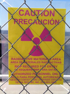
Radioactive Materials AreaRadioactivity, discovered by Madame Curie, is the process by which the nucleus of an “unstable” atom decays to a different form.  As mentioned in a previous blog post, atoms are composed of protons, neutrons and electrons; protons are easy to handle in cheminformatics, electrons are incredibly difficult and here we discuss the neutrons.

Checking whether the number of neutrons specified with an atom (the isotope) is plausible and reasonable is a non-trivial challenge.  At the most simplistic level, many cheminformatics applications and file formats ignore isotopes altogether and assume every atom has the default terrestrial isotopic composition/abundance as prescribed/recommended by IUPAC. The next level of sophistication is to treat the atomic symbols “D” and “T” as corresponding to deuterium, [2H], and tritium, [3H] respectively.

More usually, such as with MDL’s SD files or SMILES, allow the optional specification of a mass number (number of nucleons, i.e. protons+neutrons, in the nucleus).  If not specified, the element again has the IUPAC recommended composition.  A common misunderstanding with these semantics is that [12C] is not the same as [C].  Although terrestrial carbon is predominantly carbon-12 (98.89% by the latest 2009 recommendations) the presence of trace amounts of [13C] keep these distinct.  Having said that, 22 elements do have a unique isotope officially used to determine their atomic weight and hence [4Be], [9F], [11Na], [13Al], [15P], [21Sc], [25Mn], [27Co], [33As], [39Y], [41Nb], [45Rh], [53I], [55Cs], [59Pr], [65Tb], [67Ho], [69Tm], [79Au], [83Bi], [90Th] and [91Pa] may legitimately be canonicalised without the isotopic specification, i.e. [Be], F, [Na] and so on.

The most advanced cheminformatics file formats, such as Perkin Elmer Informatics’ (formerly CambridgeSoft’s) ChemDraw CDX and CDXML file format can even specify enrichment and depletion in specific isotopes. 

Unfortunately, having a specified isotope is often confused with being radioactive.  For example, RSC’s ChemSpider abuses the international icon for radioactivity to actually mean “Non-standard isotope”, though this is clearly stated.  This is because testing for a specified mass number is relatively easy, with many toolkits supporting the SMARTS semantics that [!0*] matches any specified isotope.  Although this is useful for identifying compounds whose isotopes need to be checked, it doesn’t correspond to radioactivity.  For example, deuterium, [2H] has a specified isotope but isn’t radioactive, whilst uranium, [U], even without a specified isotope is radioactive.

To address this I’ll describe how to ascertain whether a compound is radioactive, a useful descriptor especially when dealing with the “Health & Safety” parts of a pharmaceutical company.  A molecule is radioactive if any of its atoms is radioactive, and an atom is radioactive if it isn’t stable.  If an isotope isn’t specified, the element must have at least one stable isotope to be considered stable (these are the elements from hydrogen, [#1], to lead, [#82], with the exceptions of technetium [#43] and prometium [#61]), otherwise the specified isotope must correspond to one of the 255 known stable nuclides.  Hence, SMARTS pattern is_stable corresponds to [0#1,1#1,2#1,0#2,3#2,4#2,...].  Using De Morgan’s laws this atom expression can be negated to produce is_radioactive as [!0,!#1;!1,!#1;!2,!#2;…].

The complete SMARTS pattern for is_radioactive is shown below:

[!0,!#1;!1,!#1;!2,!#1;!0,!#2;!3,!#2;!4,!#2;!0,!#3;!6,!#3;!7,!#3;!0,!#4;!9,!#4;!0,!#5;!10,!#5;!11,!#5;!0,!#6;!12,!#6;!13,!#6;!0,!#7;!14,!
#7;!15,!#7;!0,!#8;!16,!#8;!17,!#8;!18,!#8;!0,!#9;!19,!#9;!0,!#10;!20,!#10;!21,!#10;!22,!#10;!0,!#11;!23,!#11;!0,!#12;!24,!#12;!25,!
#12;!26,!#12;!0,!#13;!27,!#13;!0,!#14;!28,!#14;!29,!#14;!30,!#14;!0,!#15;!31,!#15;!0,!#16;!32,!#16;!33,!#16;!34,!#16;!36,!#16;!0,
!#17;!35,!#17;!37,!#17;!0,!#18;!36,!#18;!38,!#18;!40,!#18;!0,!#19;!39,!#19;!41,!#19;!0,!#20;!40,!#20;!42,!#20;!43,!#20;!44,!#20;
!46,!#20;!0,!#21;!47,!#21;!0,!#22;!46,!#22;!47,!#22;!48,!#22;!49,!#22;!50,!#22;!0,!#23;!51,!#23;!0,!#24;!50,!#24;!52,!#24;!53,!#
24;!54,!#24;!0,!#25;!55,!#25;!0,!#26;!54,!#26;!56,!#26;!57,!#26;!58,!#26;!0,!#27;!59,!#27;!0,!#28;!58,!#28;!60,!#28;!61,!#28;!62,
!#28;!64,!#28;!0,!#29;!63,!#29;!65,!#29;!0,!#30;!64,!#30;!66,!#30;!67,!#30;!68,!#30;!70,!#30;!0,!#31;!69,!#31;!71,!#31;!0,!#32;!
70,!#32;!72,!#32;!73,!#32;!74,!#32;!0,!#33;!75,!#33;!0,!#34;!74,!#34;!76,!#34;!77,!#34;!78,!#34;!80,!#34;!0,!#35;!79,!#35;!81,!#
35;!0,!#36;!79,!#36;!80,!#36;!82,!#36;!83,!#36;!84,!#36;!86,!#36;!0,!#37;!85,!#37;!0,!#38;!84,!#38;!86,!#38;!87,!#38;!88,!#38;!0,
!#39;!89,!#39;!0,!#40;!90,!#40;!91,!#40;!92,!#40;!94,!#40;!96,!#40;!0,!#41;!93,!#41;!0,!#42;!92,!#42;!94,!#42;!95,!#42;!96,!#42;
!97,!#42;!98,!#42;!0,!#44;!96,!#44;!98,!#44;!99,!#44;!100,!#44;!101,!#44;!102,!#44;!104,!#44;!0,!#45;!103,!#45;!0,!#46;!102,!#4
6;!104,!#46;!105,!#46;!106,!#46;!108,!#46;!110,!#46;!0,!#47;!107,!#47;!109,!#47;!0,!#48;!106,!#48;!108,!#48;!110,!#48;!111,!#
48;!112,!#48;!114,!#48;!0,!#49;!113,!#49;!0,!#50;!112,!#50;!114,!#50;!115,!#50;!116,!#50;!117,!#50;!118,!#50;!119,!#50;!120,!
#50;!122,!#50;!124,!#50;!0,!#51;!121,!#51;!123,!#51;!0,!#52;!120,!#52;!122,!#52;!123,!#52;!124,!#52;!125,!#52;!126,!#52;!0,!#5
3;!127,!#53;!0,!#54;!124,!#54;!126,!#54;!128,!#54;!129,!#54;!130,!#54;!131,!#54;!132,!#54;!134,!#54;!136,!#54;!0,!#55;!133,!#
55;!0,!#56;!130,!#56;!132,!#56;!134,!#56;!135,!#56;!136,!#56;!137,!#56;!138,!#56;!0,!#57;!139,!#57;!0,!#58;!136,!#58;!138,!#5
8;!140,!#58;!142,!#58;!0,!#59;!141,!#59;!0,!#60;!142,!#60;!143,!#60;!145,!#60;!146,!#60;!148,!#60;!0,!#62;!144,!#62;!149,!#62;
!150,!#62;!152,!#62;!154,!#62;!0,!#63;!153,!#63;!0,!#64;!154,!#64;!155,!#64;!156,!#64;!157,!#64;!158,!#64;!160,!#64;!0,!#65;!1
59,!#65;!0,!#66;!156,!#66;!158,!#66;!160,!#66;!161,!#66;!162,!#66;!163,!#66;!164,!#66;!0,!#67;!165,!#67;!0,!#68;!162,!#68;!16
4,!#68;!166,!#68;!167,!#68;!168,!#68;!170,!#68;!0,!#69;!169,!#69;!0,!#70;!168,!#70;!170,!#70;!171,!#70;!172,!#70;!173,!#70;!1
74,!#70;!176,!#70;!0,!#71;!175,!#71;!0,!#72;!176,!#72;!177,!#72;!178,!#72;!179,!#72;!180,!#72;!0,!#73;!180,!#73;!181,!#73;!0,!
#74;!182,!#74;!183,!#74;!184,!#74;!186,!#74;!0,!#75;!185,!#75;!0,!#76;!184,!#76;!187,!#76;!188,!#76;!189,!#76;!190,!#76;!192,
!#76;!0,!#77;!191,!#77;!193,!#77;!0,!#78;!192,!#78;!194,!#78;!195,!#78;!196,!#78;!198,!#78;!0,!#79;!197,!#79;!0,!#80;!196,!#80
;!198,!#80;!199,!#80;!200,!#80;!201,!#80;!202,!#80;!204,!#80;!0,!#81;!203,!#81;!205,!#81;!0,!#82;!204,!#82;!206,!#82;!207,!#8
2;!208,!#82]

Image credit: LimeTech on Flickr

Patently wrong – Tracing the origin of an unusual molecule in PubChem

Greg Landrum of Novartis posted a link to PubChem structure CID60140829 on Google Plus, with the comment:

This one is from a patent with the title “Apparatus and method for encoding and decoding block low density parity check codes with a variable coding rate”. I bet it’s the result of an overly zealous (and insufficiently error checked) image->structure conversion.

A good guess, but not quite right…

First of all, let’s look at the PubChem image for the deposited structure, SID143481705 (see right). Hmmm…

These structures are from the US Patent 20050283708 via SCRIPDB. For each patent the USPTO makes available a PDF, and very usefully for chemists, the ChemDraw files associated with the patent (along with MOL, and TIFF). NextMove Software’s PatFetch (bundled with LeadMine) makes it easy to extract the corresponding PNG, CDX and MOL files for a particular structure (it runs in a web browser, and you just click on an image to obtain the CDX file). In this case, the image corresponding to the structure is as follows:
Don’t ask me what it is, but I can confirm that it’s not a crossword.

But here’s the thing. If you download the CDX file and open it in ChemDraw…you get exactly this image. 🙂 In other words, the good people at the USPTO appear to use ChemDraw as a generic drawing tool, and in particular, seem to favour carbon-carbon bonds over the actual box or line tools. Actually, now that I see how useful a grid of carbon-carbon bonds can be to create a nice table, I think I might dump Excel for good too.

Visualising a hierarchy of substructures Part II

In an earlier post, I described a simple procedure to generate a hierarchy of substructures, and depicted the hierarchy with GraphViz. Pat Walters at Vertex realised that it is possible to add images as node labels in GraphViz and updated the script so that the image includes the actual chemical depictions (see below). He has also adapted the script to use OpenEye’s OEChem.

Update (8/11/2012): Wolf-D. Ihlenfeldt has implemented this with the Cactvs Toolkit and in addition has shown how to integrate the graph display with Knime.

#!/usr/bin/env python

import copy
import pickle
import os

from openeye.oechem import *
from openeye.oedepict import *

def mol2image(mol,imageFileName,width=200,height=200):
    clearcoords = True
    suppressH   = False
    opts = OE2DMolDisplayOptions(width, height, OEScale_AutoScale)
    itf = OEInterface()
    OESetup2DMolDisplayOptions(opts, itf)
    OEPrepareDepiction(mol, clearcoords, suppressH)
    disp = OE2DMolDisplay(mol, opts)
    ofs = oeofstream(imageFileName)
    name,ext = os.path.splitext(imageFileName)
    OERenderMolecule(ofs,ext[1:],disp)

def create_tree(structures):
    tree = {"Root":{}}
    stack = [(tree["Root"], structures.keys())]

    while len(stack) > 0:
        leaf, subset = stack.pop()

        max_matches = ("", [])
        for name in subset:
            smiles = structures[name]
            smarts = OESubSearch(smiles)
            matches = []
            for nameb in subset:
                if nameb != name:
                    molb = OEGraphMol()
                    OEParseSmiles(molb,structures[nameb])
                    if smarts.SingleMatch(molb):
                        matches.append(nameb)
            if len(matches) >= len(max_matches[1]):
                max_matches = (name, matches)
        if False: # Debug statement
            print max_matches

        for name in [max_matches[0]] + max_matches[1]:
            subset.remove(name)
        leaf[max_matches[0]] = {}
        if len(subset) > 0:
            stack.append( (leaf, subset) )
        if len(max_matches[1]) > 0:
            stack.append( (leaf[max_matches[0]], copy.deepcopy(max_matches[1])))

    with open("tmp.pickle", "w") as f:
        pickle.dump(tree, f)

def fix(name):
    return name.replace("-", "_").replace("1", "one").replace("2", "two").replace("3", "three").replace("5", "five").replace(",", "_")

def visit(name, leafdict):
    for x, y in leafdict.iteritems():
        if name != "Root":
            print ' %s -> %s;' % (name,x)
        print ' %s [label=<<TABLE><TR><TD><IMG SRC="%s/%s.png"/></TD></TR></TABLE>>];' % (x,os.getcwd(),x)
        visit(x, y)

if __name__ == "__main__":
    structureDict = dict([('001', 'C(O)[C@@H](O1)[C@@H](O)[C@H](O)[C@@H](O)[CH]1(O)'),
                       ('002', 'C(O)[C@@H](O1)[C@@H](O)[C@H](O)[C@H](O)[CH]1(O)'),
                       ('003', 'C(O)[C@@H](O1)[C@@H](O)[C@H](O)[C@@H](O)[C@H]1(O)'),
                       ('004', 'C(O)[C@@H](O1)[C@@H](O)[C@H](O)[C@@H](O)[C@@H]1(O)'),
                       ('005', 'C(O)[CH](O1)[CH](O)[CH](O)[CH](O)[CH]1(O)'),
                       ('006', 'c1ccccc1'),
                       ('007', 'c1ccccc1Br'),
                       ('008', 'c1ccc(Br)cc1Br'),
                       ('009', 'c1cccc(Br)c1Br'),
                       ('010', 'c1c(Br)cc(Br)cc1Br')])

    for k in sorted(structureDict.keys()):
        imageFileName = "%s.png" % (k)
        smi = structureDict[k]
        mol = OEGraphMol()
        OEParseSmiles(mol,smi)
        mol2image(mol,imageFileName)

    create_tree(structureDict)
    with open("tmp.pickle", "r") as f:
        tree = pickle.load(f)
    print "digraph graphname {"
    print "node [shape=plaintext];"
    visit("Root", tree["Root"])
    print "}"

"""
Redirect the output to a file and then convert to a graph as follows:
"C:\Program Files (x86)\Graphviz 2.28\bin\dot.exe" -Tpng -ooutput.png dot_input.txt
"""